(s,S) Inventory System

This example is adapted (almost verbatim) from the article Kleijnen, J.P.C. et al. Constrained Optimization in Simulation: A Novel Approach, Discussion Paper 2008-95, Tilburg University, Center for Economic Research.

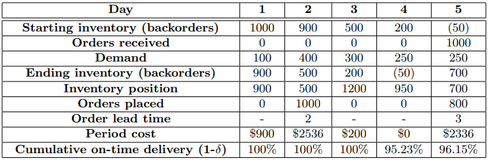
Consider a (s,S) inventory model with full backlogging. Demand during each period, \(D_t\) is distributed exponential with mean \(\mu\). At the end of each period, the inventory position \((IP_t = \text{Stock on hand} - \text{Backorders + Outstanding Orders})\) is calculated and, if it is below \(s\), an order to get back up to \(S\) is placed \((O_t = \max(\mathbb{I}(IP_t < s)(S − IP_t), 0)\). Lead times have a Poisson distribution with mean \(\theta\) days and all replenishment orders are received at the beginning of the period. Note that, since orders are placed at the end of the day, an order with lead time \(l\) placed in period \(n\) will arrive at the beginning of period \(n + l + 1\).

A per unit holding cost \(h\) is charged for inventory on-hand; furthermore, there is a fixed order cost \(f\) and a variable, per unit, cost \(c\). Our goal is to find \(s\) and \(S\) in order to minimize the \(\mathbb{E}[\text{Total cost per period}]\) such that the stockout rate \(\delta\), the fraction of demand not supplied from stock on-hand, is at most \(10\%\). To further clarify the order of events and the calculation of costs, a 5-day example in which \(s = 1000\) and \(S = 1500\), the initial inventory on hand is \(1000\) and there are no outstanding orders is provided below.

Recommended Parameter Settings: Take \(\mu = 100\), \(\theta = 6\), \(h = 1\), \(f = 36\) and \(c = 2\).

Starting Solutions: \(s = 1000\), \(S = 2000\).

If multiple solutions are needed, use \(s ∼Uniform(700,1000)\), \(S ∼Uniform(1500,2000)\).

Measurement of Time: Days simulated

Optimal Solution: Unknown